Building Dense Neural Layers

Welcome back to our course "Neural Network Fundamentals: Neurons and Layers"! You've made excellent progress so far. In the previous lessons, we built a single artificial neuron and then enhanced it with the Sigmoid activation function to introduce nonlinearity.

Today, we're taking a significant step forward in our neural networks journey. Rather than working with individual neurons, we'll learn how to group neurons together into layers — the fundamental building blocks of neural network architectures. Specifically, we'll implement a dense layer (also called a fully connected layer), which is one of the most common types of layers in neural networks.

By the end of this lesson, we'll have built a layer that can process multiple inputs through multiple neurons simultaneously, bringing us closer to implementing a complete neural network!

While a single neuron, as we've built, performs a basic computation, real-world problems demand more processing power. This is where layers come into play. A layer is essentially a group of neurons working in parallel, with each neuron in the layer processing the same input data independently. For instance, if a single neuron with 3 inputs produces 1 output, a layer of 5 such neurons, each receiving those same 3 inputs, would collectively produce 5 outputs.

This layered approach offers significant advantages:

• Increased Computational Power. Multiple neurons can learn diverse patterns from the data.
• Parallelism. All neurons in a layer compute their outputs simultaneously.
• Efficiency. Enables the use of vectorized operations (like matrix math) for faster computations.
• Hierarchical Learning. When layers are stacked, the network can learn increasingly complex features from the input.

This organization, inspired by how our brains process information, allows us to build more powerful and expressive neural network models.

One of the most fundamental and common types of layers is the dense layer, also known as a fully connected layer. Its defining characteristic is that each neuron in the layer receives input from all neurons or features of the previous layer (or the initial input data, if it's the first layer). This "full" connectivity gives it its name.

Key aspects of a dense layer include:

• Full Connectivity. Every input feature is connected to every neuron within the layer.
• Unique Parameters. Each of these connections has its own distinct weight, and each neuron in the layer has its own distinct bias.
• Shared Activation. Typically, all neurons within the same dense layer use the same activation function (like the Sigmoid we implemented).

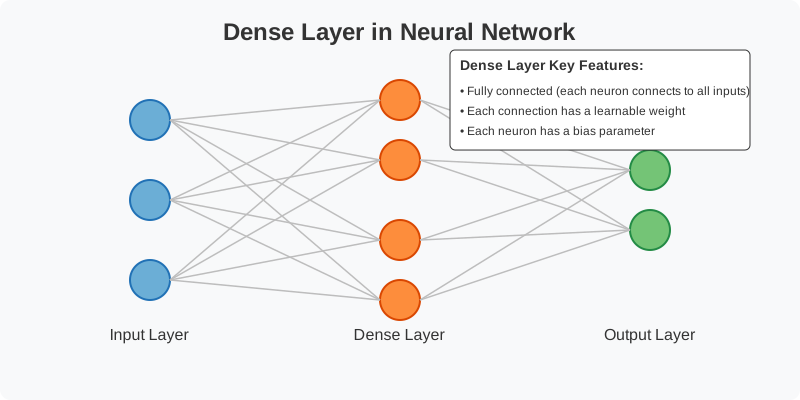
To illustrate, consider a dense layer with 4 neurons that processes an input vector containing 3 features. This configuration would result in 3 (inputs) × 4 (neurons) = 12 weight parameters and 4 bias parameters (one for each neuron in the dense layer). The layer would then produce 4 output values, one from each neuron which are fed into a final layer. In practical terms, a dense layer performs a matrix multiplication between the input and a weight matrix, adds a bias vector, and then applies an activation function to these results.

When we built a single neuron, we used basic arithmetic operations to compute the weighted sum. For a layer with multiple neurons, we can extend this approach using matrix operations, which are much more efficient than processing each neuron separately.

Let's see how we can represent the operations of a dense layer using matrices:

1. Input. A vector of size n_inputs.
2. Weights. A matrix of size n_inputs × n_neurons.
3. Biases. A vector of size n_neurons.
4. Output. A vector of size n_neurons.

The computation for the layer would be:

output = activation_function(input * weights + biases)

Where * represents matrix multiplication.

Here's a visual representation of this matrix operation for a layer with 4 inputs and 3 neurons:

Input [1×4]       Weights [4×3]         Biases [1×3]
[x₁, x₂, x₃, x₄] * [[w₁₁, w₁₂, w₁₃],   + [b₁, b₂, b₃]
                    [w₂₁, w₂₂, w₂₃],
                    [w₃₁, w₃₂, w₃₃],
                    [w₄₁, w₄₂, w₄₃]]

The result is a [1×3] vector of outputs, one from each neuron. This vectorized approach is not only more concise but also substantially faster than computing each neuron's output separately.

For our C++ implementation, we'll use 2D vectors to represent matrices and 1D vectors for our input, bias, and output vectors. This approach gives us the flexibility to perform matrix operations while keeping our code readable and maintainable.

Now that we understand the concept, let's implement our DenseLayer class. We'll start with the constructor, which initializes the weights and biases for all neurons in the layer:

#include <vector>
#include <random>
#include <iostream>

class DenseLayer {
private:
    std::vector<std::vector<double>> weights;  // 2D vector for weights matrix
    std::vector<double> biases;                // 1D vector for biases
    int n_inputs;
    int n_neurons;
    
public:
    DenseLayer(int n_inputs, int n_neurons) : n_inputs(n_inputs), n_neurons(n_neurons) {
        // Initialize random number generator
        std::random_device rd;
        std::mt19937 gen(rd());
        std::uniform_real_distribution<double> dis(0.0, 0.1);
        
        // Initialize weights matrix: shape (n_inputs, n_neurons)
        // Each row corresponds to one input, each column to one neuron
        weights.resize(n_inputs, std::vector<double>(n_neurons));
        for (int i = 0; i < n_inputs; i++) {
            for (int j = 0; j < n_neurons; j++) {
                weights[i][j] = dis(gen);  // Small random values
            }
        }
        
        // Initialize biases vector: shape (n_neurons)
        // One bias for each neuron in the layer
        biases.resize(n_neurons, 0.0);  // Initialize to zero
    }
    
    // Getter methods for accessing layer properties
    int getInputs() const { return n_inputs; }
    int getNeurons() const { return n_neurons; }
    const std::vector<std::vector<double>>& getWeights() const { return weights; }
    const std::vector<double>& getBiases() const { return biases; }
};

Here's how the initialization process works:

• The DenseLayer constructor initializes a single weight matrix and a single bias vector. These structures collectively manage the parameters for all neurons within the layer, enabling efficient, vectorized operations.
• The weights are initialized to small random values using C++'s random number generation facilities. This common practice helps break symmetry between neurons and is crucial for effective learning, preventing issues like all neurons learning the same features and aiding in the network's convergence during training.
• The biases for all neurons in the layer are initialized to zero. This provides a neutral starting point, allowing the network to learn the appropriate bias offset for each neuron based on the data during the training phase.
• Notice that our layer stores information about its dimensions (n_inputs and n_neurons), which will be useful for debugging and when connecting multiple layers together in the future.

Understanding the structure of our weights and biases is crucial for working with neural network layers. Let's examine how they're organized:

// Weights matrix: shape (n_inputs, n_neurons)
std::vector<std::vector<double>> weights;

// Biases vector: shape (n_neurons)
std::vector<double> biases;

The weights matrix has a specific organization:

• Each row represents all weights from a specific input to all neurons.
• Each column represents all weights going to a specific neuron.

For example, with 4 inputs and 3 neurons, our weights matrix might look like:

Weights [4×3]
[[0.05, 0.02, 0.08],   # Weights from input 1 to all neurons
 [0.01, 0.07, 0.03],   # Weights from input 2 to all neurons
 [0.09, 0.04, 0.06],   # Weights from input 3 to all neurons
 [0.03, 0.08, 0.01]]   # Weights from input 4 to all neurons

This structure enables efficient matrix multiplication with the input vector, computing all neuron outputs in a single operation.

The biases vector is much simpler — it's a 1D vector with one bias per neuron:

Biases [3]
[0.0, 0.0, 0.0]   # Initial biases for all three neurons

When we add this vector to the result of our matrix multiplication, each bias will be added to the corresponding neuron's computation.

Let's see our DenseLayer in action by creating and examining an instance:

int main() {
    // Example: A dense layer with 4 input features and 3 neurons
    int n_inputs_layer1 = 4;
    int n_neurons_layer1 = 3;
    DenseLayer layer1(n_inputs_layer1, n_neurons_layer1);

    std::cout << "\nInitialized Layer 1 (" << layer1.getInputs() 
              << " inputs, " << layer1.getNeurons() << " neurons):" << std::endl;
    
    // Display first 2 rows of weights matrix
    std::cout << "Layer 1 weights matrix (first 2 rows):" << std::endl;
    const auto& weights = layer1.getWeights();
    for (int i = 0; i < std::min(2, (int)weights.size()); i++) {
        std::cout << "[";
        for (int j = 0; j < weights[i].size(); j++) {
            std::cout << weights[i][j];
            if (j < weights[i].size() - 1) std::cout << ", ";
        }
        std::cout << "]" << std::endl;
    }
    std::cout << "..." << std::endl;
    
    // Display biases vector
    std::cout << "Layer 1 biases vector:" << std::endl;
    std::cout << "[";
    const auto& biases = layer1.getBiases();
    for (int i = 0; i < biases.size(); i++) {
        std::cout << biases[i];
        if (i < biases.size() - 1) std::cout << ", ";
    }
    std::cout << "]" << std::endl;

    return 0;
}

This code creates a layer that accepts 4 input features and contains 3 neurons. When we run it, we'll see:

1. A confirmation of the layer's dimensions (4 inputs, 3 neurons).
2. The first two rows of the randomly initialized weights matrix.
3. The biases vector (all zeros initially).

This simple test verifies that our layer was initialized correctly with the proper dimensions. The weights should be small random values, and the biases should all be zero.

Congratulations! You've successfully implemented a DenseLayer class that manages multiple neurons in a vectorized, efficient manner. This approach replaces our previous single-neuron implementation with a more powerful structure that can process multiple inputs through multiple neurons simultaneously. Understanding how neurons are organized into layers and how weights and biases are represented as matrices and vectors is fundamental to mastering neural networks.

In the next lesson, we'll extend our DenseLayer class by implementing the forward pass functionality. This will allow our layer to actually process input data through all neurons at once, applying the weights, biases, and activation function to transform inputs into outputs. We're steadily building toward a complete neural network implementation, and soon we'll connect multiple layers together to form deeper architectures capable of learning complex patterns in data.