Introduction

Welcome back to our course "Neural Network Fundamentals: Neurons and Layers"! In this third lesson, we're building upon what you learned in our previous lesson about the basic artificial neuron. You've already implemented a simple neuron that computes a weighted sum of inputs plus a bias.

Today, we're taking an important step forward by introducing activation functions — a crucial component that enables neural networks to learn complex patterns. In particular, we'll focus on the Sigmoid activation function, one of the classical functions used in neural networks.

In our previous lesson, our neuron could only produce linear outputs. While this is useful for some tasks, it severely limits what our neural networks can learn. Today, we'll overcome this limitation by adding non-linearity to our neurons, allowing them to model more complex relationships in data.

The Need for Non-Linearity
Understanding Activation Functions

An activation function determines whether a neuron should be "activated" or not, based on the weighted sum of its inputs.

In biological terms, this mimics how neurons in our brains "fire" when stimulated sufficiently. In computational terms, activation functions introduce non-linearity into the network, allowing it to learn complex patterns.

Activation functions typically have these characteristics:

  • They are non-linear, allowing the network to model complex relationships
  • They are differentiable, which is important for the training process (we'll explore this in future lessons)
  • They usually map inputs to a bounded range (like [0,1] or [-1,1])

Some common activation functions include:

  • Sigmoid: Maps inputs to values between 0 and 1
  • Tanh: Maps inputs to values between -1 and 1
  • ReLU (Rectified Linear Unit): Returns the input if positive; otherwise, returns 0

In this lesson, we'll focus on implementing and using the Sigmoid function, which was historically one of the first activation functions used in neural networks.

The Sigmoid Activation Function
Implementing the Sigmoid Function
Enhancing Our Neuron with Activation

Now that we have our sigmoid function, let's enhance our Neuron class from the previous lesson to include this activation function. We'll modify the forward method to apply the sigmoid function to the weighted sum:

class Neuron:
    def __init__(self, n_inputs):
        """
        Initialize a neuron.
        n_inputs: Number of input features.
        """
        self.weights = np.random.rand(n_inputs) * 0.1  # Small random weights
        self.bias = 0.0  # Start with zero bias

    def forward(self, inputs):
        """
        Calculate the neuron's output:
        1. Weighted sum of inputs and weights, plus bias.
        2. Apply the sigmoid activation function.
        inputs: A NumPy array of input features.
        """
        if inputs.shape[0] != self.weights.shape[0]:
            raise ValueError(
                f"Input size {inputs.shape[0]} does not match neuron's "
                f"expected input size {self.weights.shape[0]}."
            )
        
        weighted_sum = np.dot(inputs, self.weights)  # Calculate dot product
        raw_output = weighted_sum + self.bias  # Add bias
        
        # Apply activation function to introduce non-linearity
        activated_output = sigmoid(raw_output)
        return activated_output, raw_output  # Return both for demonstration

The key changes in this updated version are:

  1. We still calculate the weighted sum and add the bias, but now we call this intermediate result raw_output.
  2. We apply the sigmoid function to the raw output, producing an activated_output.
  3. We return both the activated output and the raw output, which will help us understand the effect of the activation function.

This two-step process — first calculating the linear combination and then applying the non-linear activation — is fundamental to how neurons operate in neural networks.

Testing the Activated Neuron

Now let's test our enhanced neuron to see how the activation function affects its output:

if __name__ == "__main__":
    # Initialize a neuron with 3 input features
    num_input_features = 3
    neuron = Neuron(num_input_features)
    print(f"Neuron weights: {neuron.weights}, Bias: {neuron.bias}")

    # Create sample input and process it through the neuron
    sample_inputs = np.array([1.0, 2.0, 3.0])
    print(f"\nInput to neuron: {sample_inputs}")
    
    # Get both raw and activated outputs
    activated_output, raw_output = neuron.forward(sample_inputs)
    print(f"Neuron's raw output (weighted sum + bias): {raw_output:.4f}")
    print(f"Neuron's activated output (Sigmoid): {activated_output:.4f}")

When we run this code, we'll observe:

  1. The random weights and bias of our initialized neuron;
  2. The input values we're feeding into the neuron;
  3. The raw output (weighted sum + bias) before applying the activation function;
  4. The final activated output after applying the sigmoid function.

Here is a sample output:

Neuron weights: [0.02619957 0.02087375 0.09072497], Bias: 0.0

Input to neuron: [1. 2. 3.]
Neuron's raw output (weighted sum + bias): 0.3401
Neuron's activated output (Sigmoid): 0.5842

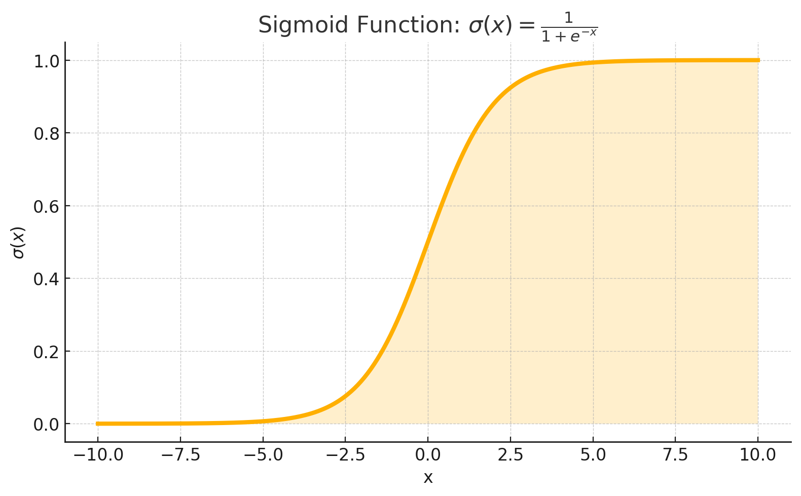
The key insight here is seeing how the sigmoid function transforms the raw output. If the raw output is a large positive number, the sigmoid output will be close to 1. If the raw output is a large negative number, the sigmoid output will be close to 0. And if the raw output is around 0, the sigmoid output will be around 0.5.

This non-linear transformation is what enables neural networks to model complex patterns and make decisions. The sigmoid function essentially "squashes" the raw output into a range between 0 and 1, which can be interpreted as a probability or a level of activation.

Conclusion and Next Steps

Excellent work! You've enhanced your neuron by adding the sigmoid activation function, introducing the critical non-linearity that neural networks need to model complex patterns. We've explored why non-linearity is essential, how the sigmoid function works mathematically, and how to implement it efficiently in code. This foundational understanding of activation functions is vital as you continue your journey into neural networks.

In the upcoming practice section, you'll gain hands-on experience working with activation functions and observe their effects on various inputs. After mastering the concepts in this lesson, we'll move forward by combining multiple neurons into layers, creating more sophisticated neural network architectures that can solve increasingly complex problems. Keep up the great work!

Sign up
Join the 1M+ learners on CodeSignal
Be a part of our community of 1M+ users who develop and demonstrate their skills on CodeSignal