Understanding LLM Costs
Introduction
Welcome to Measuring and Understanding LLM Costs in Python and to the very first unit of the course. Before we can make an LLM application cheaper, we need to know what the text-generation requests in this course cost, and that means getting comfortable with the modeled billable unit for those requests: tokens. For the text-generation requests in this course, the modeled charges are token-based, and each token category carries its own price. Production invoices may contain additional billable dimensions such as images, audio, tool execution, hosted tools, search calls, storage, fine-tuning, or provisioned throughput.
In this lesson, we will take a real API response, read the usage numbers the provider attaches to it, and convert those numbers into a calculated token cost under the rates configured in our code. One mental model will guide the whole course: provider-reported usage is the source of truth for token measurement. Billing exports or invoices remain the source of truth for actual billed cost, because discounts, rounding, service tiers, and non-token charges can affect final invoices.
The Billing Categories Behind One Request
A single request does not have a single price. The provider splits the work into categories, and each category has its own rate. Understanding these categories up front makes the code that follows much easier to read.
| Category | What it is | Typical price |
|---|---|---|
| Fresh input | Prompt tokens processed normally | Baseline input rate |
| Cache write | Prompt tokens stored for later reuse | Slight premium |
| Cached input | Prompt tokens reused from cache | Deep discount |
| Output | Tokens the model generates | Highest rate |
| Reasoning | Internal tokens, counted inside output | Output rate |
These different rates mean that two requests with the same total number of tokens can still have different costs.
How the Token Categories Fit Together
Input tokens are divided into fresh input, cache-write, and cached-input categories. Reasoning tokens are different: they are already included within the output-token total rather than added as a separate billing category.
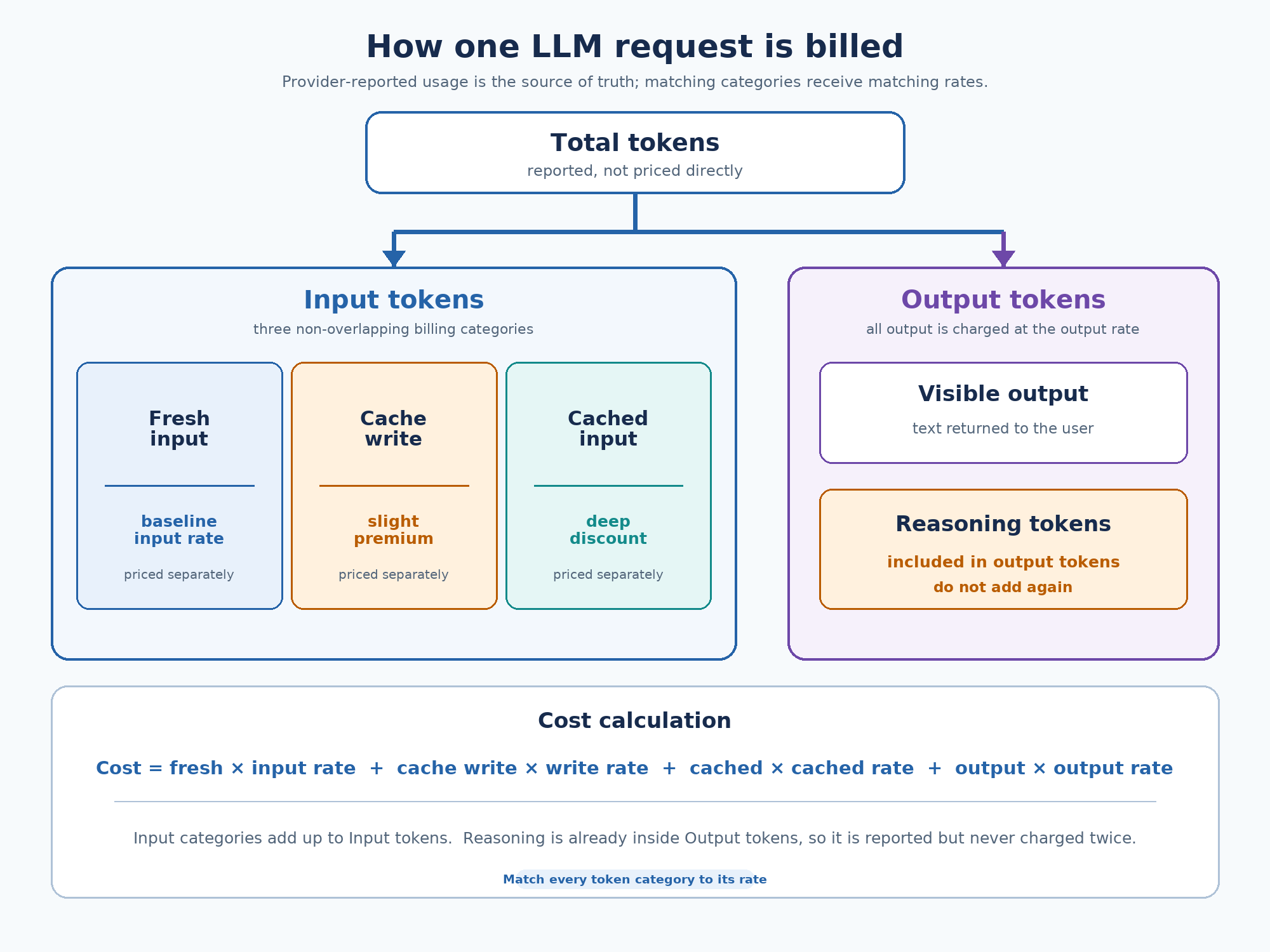
Notice that output is usually the most expensive category, often several times the input rate. That single fact will shape many optimization decisions later in this path.
Setting Up the Call: Model and Per-Token Rates
Let us start at the top of the file, where we declare which model we are calling and what each token type costs us.
Providers publish pricing per million tokens because per-token prices are awkwardly small. Dividing once at the top keeps the rest of the math simple: every later line is just tokens * rate. Keeping these values in named constants, rather than sprinkling raw numbers throughout the cost formula, is a habit that pays off in Unit 3, when we wrap all of this into a reusable cost layer.
The rates in this course reflect OpenAI’s standard GPT-5.6 Luna API pricing as checked on August 11, 2026: $1.00 per million fresh-input tokens, $1.25 per million cache-write tokens, $0.10 per million cached-input tokens, and $6.00 per million output tokens. These rates apply to standard processing for context lengths below 270K tokens. API pricing can change, so verify OpenAI’s current pricing before using these constants in production.
Making the Request and Finding the Usage Object
Now we send a real request and look at what comes back.
The response object carries two things we care about, and they serve very different purposes:
response.output_textis the answer we show to a user.response.usageis the record we are billed for.
Inside usage, three top-level counters are available: usage.input_tokens, usage.output_tokens, and usage.total_tokens. The first two are the ones that drive costs. total_tokens is simply their sum, offered as a convenience; it is never priced on its own, so we report it but never multiply it by a rate.
Inside the Input: Fresh, Cached, and Cache-Write Tokens
Here is the first subtlety: usage.input_tokens is a single total that can hide three differently priced groups. The provider exposes the special cases in a details object, and we derive the rest.
The provider reports the total plus the two exceptional buckets, so anything left over is ordinary, full-price input. Subtraction gives us that remainder safely, and the three parts always add back up to usage.input_tokens.
Intuitively:
- Fresh input: processed from scratch, charged at the normal rate.
- Cache write: a stable prompt prefix being stored, charged at a small premium.
- Cached input: that prefix reused on a later call, charged at a deep discount.
That premium-now-for-discount-later tradeoff is exactly what we explore in a later course of this path.
Inside the Output: Visible Text and Reasoning Tokens
The output side has its own hidden detail. Reasoning-capable models generate internal tokens while working through a problem, and those tokens never appear in output_text.
The critical billing point is this: reasoning tokens are already included in usage.output_tokens, and they are billed at the output rate. We read them so we can report them, not so we can add them again. Adding reasoning_tokens on top of output_tokens is one of the most common ways a cost calculation quietly overcharges.
Practically, this explains a confusing experience many teams have: a model returns three short sentences, yet the bill looks large. The visible answer was small, but hundreds of reasoning tokens were generated and charged along the way.
Turning Usage Into Dollars
With every category separated, the cost formula becomes a direct translation of "tokens times matching rate."
The central lesson of this unit lives in that comment: we cannot multiply usage.input_tokens by a single input rate, because one total can mix three prices. For our sample run, with 19 fresh input tokens and 32 output tokens and nothing cached:
Two bugs to watch for: charging all input at the fresh rate (which erases every dollar of cache savings from your reports) and double-counting reasoning tokens on top of output tokens.
Reporting the Breakdown Clearly
Finally, we print the answer and the numbers behind it, with indentation showing which counts nest inside which totals.
The ${cost:.6f} format matters more than it looks: a single call often costs a small fraction of a cent, and fewer decimals would round our result straight down to $0.00. Running the full program gives us:
The breakdown, not the single total, is what later tells us which category to attack.
Conclusion and Next Steps
We now have a complete measurement pipeline: make a call, read usage, split the input into fresh, cache-write, and cached tokens, separate reasoning inside the output, apply each matching rate, and report the calculated token cost clearly. The takeaway to carry forward is that provider-reported usage is our token-usage source of truth; configured rates let us calculate comparable token costs, while actual billed cost still requires a provider billing export or invoice reconciliation.
In the practice exercises ahead, we will read usage numbers, split input into billing categories, calculate the configured-rate token cost, and change prompts to compare how usage shifts. Once measuring feels natural, Unit 2 flips the timing: estimating cost before the call, then checking how close the guess was.
Time to open the editor and put these numbers to work.
