Welcome to the fifth and final lesson in Fitting a Line to Data! Over the previous four lessons, you built a complete toolkit: you assigned explanatory and response roles, summarized a trend with a straight line, measured individual prediction errors with residuals, and rolled those residuals into a single total squared error score. Each step gave us a sharper way to evaluate how well a line fits a scatter plot.
Now we bring everything together. In this lesson, you will discover that among every possible line you could draw through a scatter plot, exactly one earns the lowest total squared error. We will learn what this special line is called, express it as a simple equation, and explore a remarkable property it always has. Let's meet the least-squares regression line.
From Scoring Lines to Finding the Best One
In the previous lesson, you compared two candidate lines by computing each line's total squared error and picking the smaller score. That approach works perfectly when you only have two options on the table. But a scatter plot does not come with just two choices — there are infinitely many straight lines you could draw through the data, each with a different slope and position.
Imagine you could somehow test every one of those lines, calculating the total squared error for each. Some lines would score terribly, some would score reasonably well, and one would score the very best. Because total squared error is a smooth quantity that changes predictably as you tilt and shift a line, that "best score" is not a tie; it belongs to a single line. That is the concept we will make precise in the next section.
The Least-Squares Regression Line
Among all the infinitely many straight lines we could draw through a scatter plot, exactly one produces the smallest possible total squared error. This unique line is called the least-squares regression line.
The name tells the story: "least squares" means it minimizes the sum of squared residuals. No other straight line can beat its score. The good news is that we do not have to test millions of lines by hand. Mathematicians have worked out formulas that jump directly to the winning line using the data. The least-squares regression line is not a guess or a rough estimate — it is the mathematically determined best-fit line for a given data set.
Join the 1M+ learners on CodeSignal
Be a part of our community of 1M+ users who develop and demonstrate their skills on CodeSignal
If you remember the equation of a line from algebra class, the statistics version might look a bit backwards. It is helpful to compare them side-by-side:
Feature
Algebra Notation
Statistics Notation
Standard Equation
y=mx+b
y^=a+bx
Slope
m
b
Y-intercept
b
a
In statistics, we use b for the slope because it represents the coefficient of the x variable. While the letters change, the mechanics remain the same: the slope tells you the rate of change, and the intercept tells you where the line hits the vertical axis.
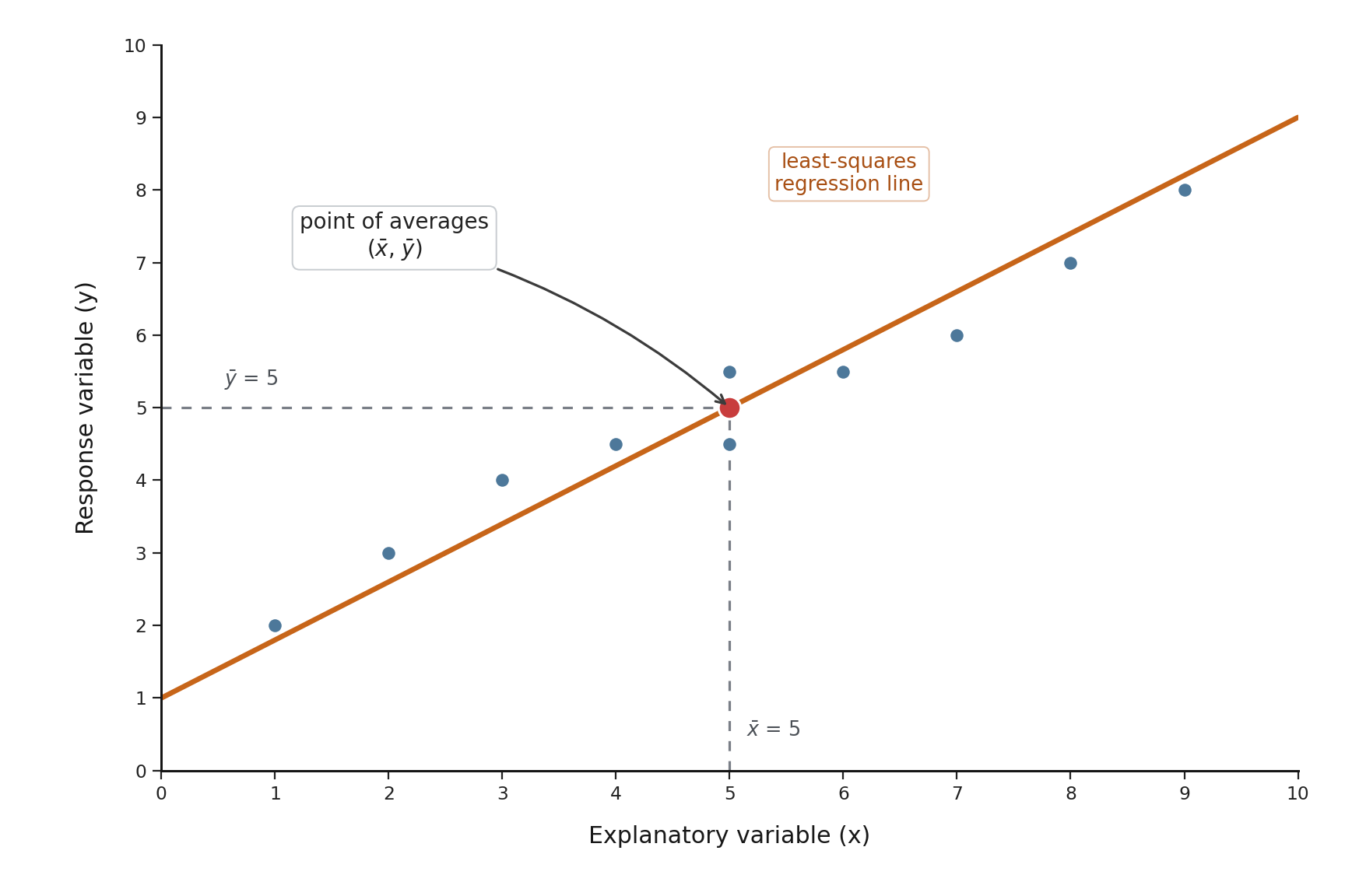
Regardless of the notation, the least-squares line is always mathematically tethered to the data. It must pass through the point of averages (xˉ,yˉ). You can think of this point as the Anchor Point or the Center of Gravity of the scatter plot; the line can tilt to find the best slope, but it must pivot through this specific center.
Like any straight line, the least-squares regression line can be written as a linear equation:
y^=a+bx
Here x is a value of the explanatory variable, and y^ (read "y-hat") is the predicted value of the response variable. The letter b is the slope, and a is the y-intercept. The hat symbol on y is a reminder that we are talking about a prediction from the line, not an actual observed data value.
Both a and b are calculated entirely from the data. You may recall from earlier in this learning path that we worked with means (xˉ and yˉ), standard deviations (sx and sy), and the correlation coefficient (r). The slope of the least-squares line ties all of these together:
b=r⋅sxsy
Once we know the slope, the intercept follows from a short formula we will see in the next section. The important takeaway is that every number in the equation comes straight from the data, so a different data set will always produce a different line.
The least-squares regression line has a property that holds for every data set: it always passes through the point (xˉ,yˉ), where xˉ is the mean of the explanatory variable and yˉ is the mean of the response variable. As mentioned, this Anchor Point sits right at the center of the data cloud.
Why does this make sense? The regression line is meant to capture the overall trend, and the center of that trend naturally lives at the average of both variables. This guaranteed property also gives us a clean way to calculate the intercept once we know the slope:
a=yˉ−bxˉ
The scatter plot below illustrates this idea. While many lines could pass through this highlighted average point, only the least-squares line does so while also minimizing the total squared error for the entire data set:
In other words, once the slope is set by the correlation and standard deviations, the intercept is the specific value that forces the line through the point of averages. This is a guaranteed feature of the least-squares method.
Let's connect all of these ideas with a worked example. Suppose a coffee-shop manager collects data on afternoon temperature (explanatory) and iced-coffee sales (response). From her data, she calculates:
xˉ=20 (mean temperature in °C), yˉ=50 (mean iced coffees sold)
r=0.8, sx=4, sy=10
Step 1: Calculate the Slope (b)
b=r⋅sxsy=0.8⋅410=2.0
Step 2: Calculate the Intercept (a)
Using the property that the line must pass through (xˉ,yˉ):
a=yˉ−bxˉ=50−(2.0⋅20)=50−40=10
Equation of the least-squares line:
y^=10+2.0x
We can verify the average-point property by plugging in the mean temperature x=20: we get y^=10+2.0(20)=50, which is exactly the mean sales yˉ. The line passes right through (20,50), just as the theory promises. The key takeaway is that the data alone — its means, standard deviations, and correlation — determined every part of this unique "best-fit" equation.
In this lesson, you learned that among all possible lines, exactly one minimizes the total squared error — the least-squares regression line. This line is expressed as the linear equation y^=a+bx, with its slope and intercept calculated from the data's means, standard deviations, and correlation. A defining property of this line is that it always passes through the point of averages(xˉ,yˉ), anchoring it to the very center of the data.
Now it is your turn to put these ideas into practice! In the upcoming exercises, you will pin down the defining properties of the least-squares line, separate fact from common misconceptions, experiment with adjusting a line to find the best fit interactively, and explain in your own words how the data determines this special line. Jump in and show what you have learned!