Too Close to Call
Introduction
Every prediction rests on a simple bet: that the pattern we see in a sample reflects what is truly happening in the population. But what happens when the race is almost a dead heat — say, versus ? Should we still declare a winner, or should we hold back? Welcome to the seventh and final lesson of Drawing Conclusions from a Sample, where we tackle one of the most important judgment calls in statistics: recognizing when sample results are too close to call.
When the Numbers Are Nearly Even
Picture a company that surveys a random sample of 200 customers, asking whether they prefer a redesigned logo (Design A) or the current one (Design B). The results come back: 104 choose Design A and 96 choose Design B. Design A is ahead with a proportion of against for Design B.
Should the company announce that most customers prefer the new logo? The margin here is razor-thin. As you learned earlier in this course, every random sample produces a slightly different set of estimates. If we drew a different random sample of 200, Design B might come out ahead instead. Before making a prediction, we need to ask whether the gap we observe is real or whether it could simply be the result of ordinary sampling variation.
Sampling Variation Can Flip the Leader
Recall that repeated random samples produce estimates that cluster around the true population value but vary from sample to sample. We also learned to gauge the likely error by looking at how spread out those sample estimates tend to be. That same reasoning applies directly when two options are competing.
If the true population is split close to evenly, then some samples will show Option A ahead while other samples of the exact same size will show Option B ahead. The smaller the gap in our sample result, the more plausible it becomes that the gap is simply noise rather than a genuine population-level difference. In other words, a tiny lead in one sample does not guarantee a lead in the next sample — or in the population.
A Clear Lead vs. a Near-Tie
One helpful way to judge whether a lead is trustworthy is to use the plausible range as a rough check on the leading option's true proportion. If that range stays comfortably above , we have stronger evidence for a population prediction. If it dips below , a different sample could easily reverse the result, so we should be cautious.
Let's compare two scenarios, both using a random sample of 200 customers choosing between Option A and Option B.
Scenario 1 — A clear lead
| Option | Count | Sample Proportion |
|---|---|---|
| A | 134 | |
| B | 66 |
The gap is . Even after accounting for sampling variation, the plausible range for Option A's true proportion stays well above . We can confidently predict that Option A is preferred in the population.
Scenario 2 — A near-tie
| Option | Count | Sample Proportion |
|---|---|---|
| A | 104 | |
| B | 96 |
The gap is only . For a sample of 200, the plausible range for Option A's true proportion could easily include values below . A different random sample might well show Option B in the lead. This result is too close to call.
The illustration below shows this contrast using plausible ranges around each sample proportion:
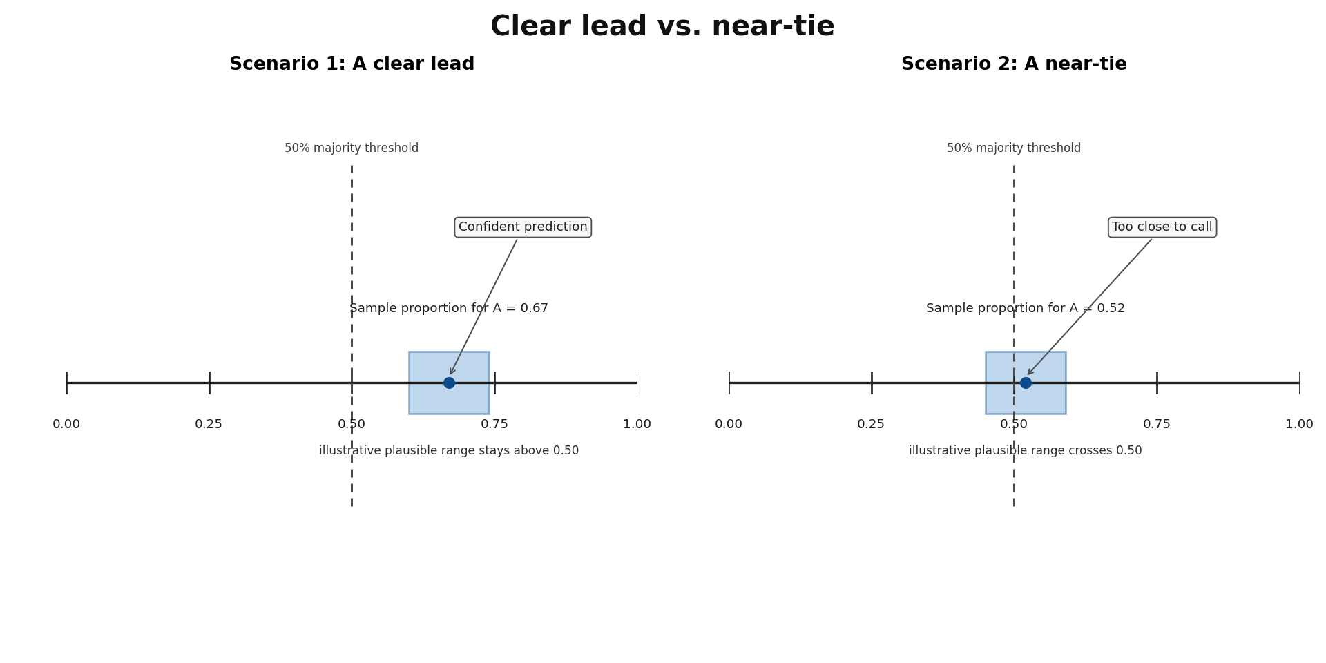
In Scenario 1, the plausible range for Option A sits entirely above , so the sample gives stronger evidence for Option A. In Scenario 2, the range crosses , meaning sampling variation alone could put either option on top and the evidence is too weak for a confident call.
