Modular Training Components

Introduction

Welcome back to lesson 2 of "Building and Applying Your Neural Network Library"! You've made excellent progress in this course. In our previous lesson, we successfully transformed our neural network code into a well-structured C++ library by modularizing our core components — dense layers and activation functions . We created clean include paths and established the foundation for a professional-grade neural network library using proper header and source file organization. Now we're ready to take the next crucial step: modularizing our training components . As you may recall from our previous courses, training a neural network involves two key components beyond the layers themselves: loss functions (which measure how well our network is performing) and optimizers (which update the network's weights based on the gradients we compute). Currently, these components are scattered throughout our training code, making them difficult to reuse and maintain. In this lesson, we'll organize these training components into dedicated namespaces within our neuralnets library. We'll create a losses namespace to house our mean squared error (MSE) loss function and an optimizers namespace for our stochastic gradient descent (SGD) optimizer. By the end of this lesson, you'll have a complete, modular training pipeline that demonstrates the power of good software architecture in machine learning projects.

Our Test Dataset: The XOR Problem

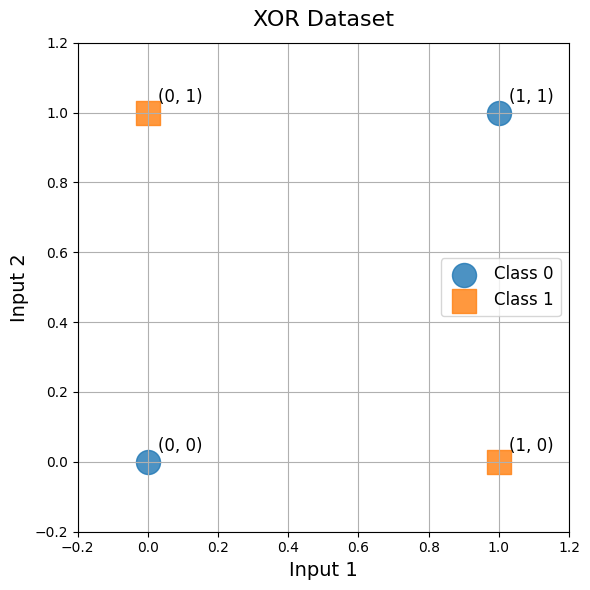
Before we dive into modularizing our training components, let's take a moment to understand the dataset we'll be using to test our library: the XOR (exclusive OR) problem . This is a classic toy problem in machine learning that serves as an excellent test case for neural networks because it's non-linearly separable — meaning a single linear classifier cannot solve it, but a simple multi-layer neural network can. The XOR problem consists of four data points with two binary inputs and one binary output. The output is 1 when exactly one of the inputs is 1, and 0 otherwise. This creates the pattern: [0,0] \to 0, [0,1] \to 1, [1,0] \to 1, [1,1] \to 0 . This is typically treated as a classification problem, but we can frame it as a regression task as well, which is what we'll do by using our mse loss. Despite its simplicity, if our network can learn XOR, then we know our forward pass, backward pass, loss calculation, and optimization code are all functioning properly. C++ // XOR dataset setup using Eigen matrices Eigen::MatrixXd X_train(4, 2); X_train << 0, 0, 0, 1, 1, 0, 1, 1; Eigen::MatrixXd y_train(4, 1); y_train << 0, 1, 1, 0; // XOR dataset setup using Eigen matrices Eigen::MatrixXd X_train(4, 2); X_train << 0, 0, 0, 1, 1, 0, 1, 1; Eigen::MatrixXd y_train(4, 1); y_train << 0, 1, 1, 0; While we're using XOR for rapid development and testing in this lesson, later in the course we'll apply our complete neural network library to a real-world dataset — the California housing dataset — where we'll predict house prices based on various features like location, population, and median income.

Join the 1M+ learners on CodeSignal

Be a part of our community of 1M+ users who develop and demonstrate their skills on CodeSignal

C++

// XOR dataset setup using Eigen matrices
Eigen::MatrixXd X_train(4, 2);
X_train << 0, 0,
           0, 1,
           1, 0,
           1, 1;

Eigen::MatrixXd y_train(4, 1);
y_train << 0,
           1,
           1,
           0;

C++

#ifndef NEURALNETS_LOSSES_MSE_HPP
#define NEURALNETS_LOSSES_MSE_HPP

#include <Eigen/Dense>

namespace neuralnets {
namespace losses {

/**
 * Calculate Mean Squared Error loss.
 * @param y_true True target values
 * @param y_pred Predicted values
 * @return MSE loss value
 */
double mse_loss(const Eigen::MatrixXd& y_true, const Eigen::MatrixXd& y_pred);

/**
 * Derivative of MSE loss w.r.t. y_pred.
 * @param y_true True target values
 * @param y_pred Predicted values
 * @return Gradient matrix
 */
Eigen::MatrixXd mse_loss_derivative(const Eigen::MatrixXd& y_true, const Eigen::MatrixXd& y_pred);

} // namespace losses
} // namespace neuralnets

#endif // NEURALNETS_LOSSES_MSE_HPP

#ifndef NEURALNETS_LOSSES_MSE_HPP
#define NEURALNETS_LOSSES_MSE_HPP

#include <Eigen/Dense>

namespace neuralnets {
namespace losses {

/**
 * Calculate Mean Squared Error loss.
 * @param y_true True target values
 * @param y_pred Predicted values
 * @return MSE loss value
 */
double mse_loss(const Eigen::MatrixXd& y_true, const Eigen::MatrixXd& y_pred);

/**
 * Derivative of MSE loss w.r.t. y_pred.
 * @param y_true True target values
 * @param y_pred Predicted values
 * @return Gradient matrix
 */
Eigen::MatrixXd mse_loss_derivative(const Eigen::MatrixXd& y_true, const Eigen::MatrixXd& y_pred);

} // namespace losses
} // namespace neuralnets

#endif // NEURALNETS_LOSSES_MSE_HPP

C++

#include "neuralnets/losses/mse.hpp"

namespace neuralnets {
namespace losses {

double mse_loss(const Eigen::MatrixXd& y_true, const Eigen::MatrixXd& y_pred) {
    Eigen::MatrixXd diff = y_true - y_pred;
    return diff.array().square().mean();
}

Eigen::MatrixXd mse_loss_derivative(const Eigen::MatrixXd& y_true, const Eigen::MatrixXd& y_pred) {
    // Normalize by batch size (number of samples)
    return 2.0 * (y_pred - y_true) / y_true.rows();
}

} // namespace losses
} // namespace neuralnets

#include "neuralnets/losses/mse.hpp"

namespace neuralnets {
namespace losses {

double mse_loss(const Eigen::MatrixXd& y_true, const Eigen::MatrixXd& y_pred) {
    Eigen::MatrixXd diff = y_true - y_pred;
    return diff.array().square().mean();
}

Eigen::MatrixXd mse_loss_derivative(const Eigen::MatrixXd& y_true, const Eigen::MatrixXd& y_pred) {
    // Normalize by batch size (number of samples)
    return 2.0 * (y_pred - y_true) / y_true.rows();
}

} // namespace losses
} // namespace neuralnets

C++

#ifndef NEURALNETS_OPTIMIZERS_SGD_HPP
#define NEURALNETS_OPTIMIZERS_SGD_HPP

#include "neuralnets/layers/dense.hpp"

namespace neuralnets {
namespace optimizers {

class SGD {
private:
    double learning_rate_;

public:
    /**
     * Constructor for SGD optimizer.
     * @param learning_rate Learning rate for weight updates
     */
    explicit SGD(double learning_rate = 0.01);

    /**
     * Update layer's weights and biases using stored gradients.
     * @param layer Reference to the layer to update
     */
    void update(layers::DenseLayer& layer);
};

} // namespace optimizers
} // namespace neuralnets

#endif // NEURALNETS_OPTIMIZERS_SGD_HPP

#ifndef NEURALNETS_OPTIMIZERS_SGD_HPP
#define NEURALNETS_OPTIMIZERS_SGD_HPP

#include "neuralnets/layers/dense.hpp"

namespace neuralnets {
namespace optimizers {

class SGD {
private:
    double learning_rate_;

public:
    /**
     * Constructor for SGD optimizer.
     * @param learning_rate Learning rate for weight updates
     */
    explicit SGD(double learning_rate = 0.01);

    /**
     * Update layer's weights and biases using stored gradients.
     * @param layer Reference to the layer to update
     */
    void update(layers::DenseLayer& layer);
};

} // namespace optimizers
} // namespace neuralnets

#endif // NEURALNETS_OPTIMIZERS_SGD_HPP

C++

#include "neuralnets/optimizers/sgd.hpp"

namespace neuralnets {
namespace optimizers {

SGD::SGD(double learning_rate) : learning_rate_(learning_rate) {}

void SGD::update(layers::DenseLayer& layer) {
    // Update weights and biases using stored gradients
    if (layer.has_gradients()) {
        layer.weights_ -= learning_rate_ * layer.d_weights_;
        layer.biases_ -= learning_rate_ * layer.d_biases_;
    }
}

} // namespace optimizers
} // namespace neuralnets

#include "neuralnets/optimizers/sgd.hpp"

namespace neuralnets {
namespace optimizers {

SGD::SGD(double learning_rate) : learning_rate_(learning_rate) {}

void SGD::update(layers::DenseLayer& layer) {
    // Update weights and biases using stored gradients
    if (layer.has_gradients()) {
        layer.weights_ -= learning_rate_ * layer.d_weights_;
        layer.biases_ -= learning_rate_ * layer.d_biases_;
    }
}

} // namespace optimizers
} // namespace neuralnets

C++

#include <iostream>
#include <iomanip>
#include <Eigen/Dense>
#include "neuralnets/layers/dense.hpp"
#include "neuralnets/losses/mse.hpp"
#include "neuralnets/optimizers/sgd.hpp"

using namespace neuralnets;

int main() {
    // Sample data: XOR problem
    Eigen::MatrixXd X_train(4, 2);
    X_train << 0, 0,
               0, 1,
               1, 0,
               1, 1;

    Eigen::MatrixXd y_train(4, 1);
    y_train << 0,
               1,
               1,
               0;

    // Build MLP using modular components
    MLP mlp;
    mlp.add_layer(std::make_unique<layers::DenseLayer>(2, 4, "relu"));
    mlp.add_layer(std::make_unique<layers::DenseLayer>(4, 1, "sigmoid"));

    // Use modular optimizer
    optimizers::SGD optimizer(0.5);

    // Training loop
    int epochs = 1000;
    std::cout << "Training MLP for XOR problem for " << epochs 
              << " epochs with LR=0.5" << std::endl;

    for (int epoch = 0; epoch < epochs; ++epoch) {
        // 1. Forward pass
        Eigen::MatrixXd y_pred = mlp.forward(X_train);
        
        // 2. Calculate loss using modular loss function
        double loss = losses::mse_loss(y_train, y_pred);
        
        // 3. Calculate gradient using modular derivative
        Eigen::MatrixXd d_loss_wrt_pred = losses::mse_loss_derivative(y_train, y_pred);
        
        // 4. Backward pass through network
        mlp.backward(d_loss_wrt_pred);
        
        // 5. Update weights using modular optimizer
        for (auto& layer : mlp.get_layers()) {
            optimizer.update(*layer);
        }
        
        if ((epoch + 1) % 200 == 0 || epoch == 0) {
            std::cout << "Epoch " << std::setw(4) << (epoch + 1) << "/" << epochs 
                      << ", Loss: " << std::fixed << std::setprecision(6) << loss << std::endl;
        }
    }

    // Test final performance
    std::cout << "\n--- After Training ---" << std::endl;
    Eigen::MatrixXd final_preds = mlp.forward(X_train);
    std::cout << "Input | True Output | Predicted Output | Rounded Prediction" << std::endl;
    
    for (int i = 0; i < X_train.rows(); ++i) {
        double pred_val = final_preds(i, 0);
        int rounded_pred = static_cast<int>(std::round(pred_val));
        
        std::cout << "[" << X_train(i, 0) << " " << X_train(i, 1) << "] | " 
                  << std::setw(11) << static_cast<int>(y_train(i, 0)) << " | " 
                  << std::setw(16) << std::fixed << std::setprecision(4) << pred_val << " | " 
                  << std::setw(18) << rounded_pred << std::endl;
    }

    return 0;
}

#include <iostream>
#include <iomanip>
#include <Eigen/Dense>
#include "neuralnets/layers/dense.hpp"
#include "neuralnets/losses/mse.hpp"
#include "neuralnets/optimizers/sgd.hpp"

using namespace neuralnets;

int main() {
    // Sample data: XOR problem
    Eigen::MatrixXd X_train(4, 2);
    X_train << 0, 0,
               0, 1,
               1, 0,
               1, 1;

    Eigen::MatrixXd y_train(4, 1);
    y_train << 0,
               1,
               1,
               0;

    // Build MLP using modular components
    MLP mlp;
    mlp.add_layer(std::make_unique<layers::DenseLayer>(2, 4, "relu"));
    mlp.add_layer(std::make_unique<layers::DenseLayer>(4, 1, "sigmoid"));

    // Use modular optimizer
    optimizers::SGD optimizer(0.5);

    // Training loop
    int epochs = 1000;
    std::cout << "Training MLP for XOR problem for " << epochs 
              << " epochs with LR=0.5" << std::endl;

    for (int epoch = 0; epoch < epochs; ++epoch) {
        // 1. Forward pass
        Eigen::MatrixXd y_pred = mlp.forward(X_train);
        
        // 2. Calculate loss using modular loss function
        double loss = losses::mse_loss(y_train, y_pred);
        
        // 3. Calculate gradient using modular derivative
        Eigen::MatrixXd d_loss_wrt_pred = losses::mse_loss_derivative(y_train, y_pred);
        
        // 4. Backward pass through network
        mlp.backward(d_loss_wrt_pred);
        
        // 5. Update weights using modular optimizer
        for (auto& layer : mlp.get_layers()) {
            optimizer.update(*layer);
        }
        
        if ((epoch + 1) % 200 == 0 || epoch == 0) {
            std::cout << "Epoch " << std::setw(4) << (epoch + 1) << "/" << epochs 
                      << ", Loss: " << std::fixed << std::setprecision(6) << loss << std::endl;
        }
    }

    // Test final performance
    std::cout << "\n--- After Training ---" << std::endl;
    Eigen::MatrixXd final_preds = mlp.forward(X_train);
    std::cout << "Input | True Output | Predicted Output | Rounded Prediction" << std::endl;
    
    for (int i = 0; i < X_train.rows(); ++i) {
        double pred_val = final_preds(i, 0);
        int rounded_pred = static_cast<int>(std::round(pred_val));
        
        std::cout << "[" << X_train(i, 0) << " " << X_train(i, 1) << "] | " 
                  << std::setw(11) << static_cast<int>(y_train(i, 0)) << " | " 
                  << std::setw(16) << std::fixed << std::setprecision(4) << pred_val << " | " 
                  << std::setw(18) << rounded_pred << std::endl;
    }

    return 0;
}

cmake

cmake_minimum_required(VERSION 3.10)
project(NeuralNets)

set(CMAKE_CXX_STANDARD 17)

# Find Eigen3
find_package(Eigen3 REQUIRED)

# Include directories
include_directories(include)

# Source files
set(SOURCES
    src/layers/dense.cpp
    src/losses/mse.cpp
    src/optimizers/sgd.cpp
    src/main.cpp
)

# Create executable
add_executable(neuralnets ${SOURCES})

# Link Eigen3
target_link_libraries(neuralnets Eigen3::Eigen)

cmake_minimum_required(VERSION 3.10)
project(NeuralNets)

set(CMAKE_CXX_STANDARD 17)

# Find Eigen3
find_package(Eigen3 REQUIRED)

# Include directories
include_directories(include)

# Source files
set(SOURCES
    src/layers/dense.cpp
    src/losses/mse.cpp
    src/optimizers/sgd.cpp
    src/main.cpp
)

# Create executable
add_executable(neuralnets ${SOURCES})

# Link Eigen3
target_link_libraries(neuralnets Eigen3::Eigen)

Shell

mkdir build && cd build
cmake ..
make
./neuralnets

mkdir build && cd build
cmake ..
make
./neuralnets

text

Training MLP for XOR problem for 1000 epochs with LR=0.5
Epoch    1/1000, Loss: 0.250048
Epoch  200/1000, Loss: 0.036447
Epoch  400/1000, Loss: 0.006105
Epoch  600/1000, Loss: 0.002965
Epoch  800/1000, Loss: 0.001892
Epoch 1000/1000, Loss: 0.001377

--- After Training ---
Input | True Output | Predicted Output | Rounded Prediction
[0 0] |           0 |           0.0580 |                  0
[0 1] |           1 |           0.9745 |                  1
[1 0] |           1 |           0.9748 |                  1
[1 1] |           0 |           0.0291 |                  0

Training MLP for XOR problem for 1000 epochs with LR=0.5
Epoch    1/1000, Loss: 0.250048
Epoch  200/1000, Loss: 0.036447
Epoch  400/1000, Loss: 0.006105
Epoch  600/1000, Loss: 0.002965
Epoch  800/1000, Loss: 0.001892
Epoch 1000/1000, Loss: 0.001377

--- After Training ---
Input | True Output | Predicted Output | Rounded Prediction
[0 0] |           0 |           0.0580 |                  0
[0 1] |           1 |           0.9745 |                  1
[1 0] |           1 |           0.9748 |                  1
[1 1] |           0 |           0.0291 |                  0

C++

#ifndef NEURALNETS_LOSSES_MSE_HPP
#define NEURALNETS_LOSSES_MSE_HPP

#include <Eigen/Dense>

namespace neuralnets {
namespace losses {

/**
 * Calculate Mean Squared Error loss.
 * @param y_true True target values
 * @param y_pred Predicted values
 * @return MSE loss value
 */
double mse_loss(const Eigen::MatrixXd& y_true, const Eigen::MatrixXd& y_pred);

/**
 * Derivative of MSE loss w.r.t. y_pred.
 * @param y_true True target values
 * @param y_pred Predicted values
 * @return Gradient matrix
 */
Eigen::MatrixXd mse_loss_derivative(const Eigen::MatrixXd& y_true, const Eigen::MatrixXd& y_pred);

} // namespace losses
} // namespace neuralnets

#endif // NEURALNETS_LOSSES_MSE_HPP

C++

#include "neuralnets/losses/mse.hpp"

namespace neuralnets {
namespace losses {

double mse_loss(const Eigen::MatrixXd& y_true, const Eigen::MatrixXd& y_pred) {
    Eigen::MatrixXd diff = y_true - y_pred;
    return diff.array().square().mean();
}

Eigen::MatrixXd mse_loss_derivative(const Eigen::MatrixXd& y_true, const Eigen::MatrixXd& y_pred) {
    // Normalize by batch size (number of samples)
    return 2.0 * (y_pred - y_true) / y_true.rows();
}

} // namespace losses
} // namespace neuralnets

C++

#ifndef NEURALNETS_OPTIMIZERS_SGD_HPP
#define NEURALNETS_OPTIMIZERS_SGD_HPP

#include "neuralnets/layers/dense.hpp"

namespace neuralnets {
namespace optimizers {

class SGD {
private:
    double learning_rate_;

public:
    /**
     * Constructor for SGD optimizer.
     * @param learning_rate Learning rate for weight updates
     */
    explicit SGD(double learning_rate = 0.01);

    /**
     * Update layer's weights and biases using stored gradients.
     * @param layer Reference to the layer to update
     */
    void update(layers::DenseLayer& layer);
};

} // namespace optimizers
} // namespace neuralnets

#endif // NEURALNETS_OPTIMIZERS_SGD_HPP

C++

#include "neuralnets/optimizers/sgd.hpp"

namespace neuralnets {
namespace optimizers {

SGD::SGD(double learning_rate) : learning_rate_(learning_rate) {}

void SGD::update(layers::DenseLayer& layer) {
    // Update weights and biases using stored gradients
    if (layer.has_gradients()) {
        layer.weights_ -= learning_rate_ * layer.d_weights_;
        layer.biases_ -= learning_rate_ * layer.d_biases_;
    }
}

} // namespace optimizers
} // namespace neuralnets

C++

#include <iostream>
#include <iomanip>
#include <Eigen/Dense>
#include "neuralnets/layers/dense.hpp"
#include "neuralnets/losses/mse.hpp"
#include "neuralnets/optimizers/sgd.hpp"

using namespace neuralnets;

int main() {
    // Sample data: XOR problem
    Eigen::MatrixXd X_train(4, 2);
    X_train << 0, 0,
               0, 1,
               1, 0,
               1, 1;

    Eigen::MatrixXd y_train(4, 1);
    y_train << 0,
               1,
               1,
               0;

    // Build MLP using modular components
    MLP mlp;
    mlp.add_layer(std::make_unique<layers::DenseLayer>(2, 4, "relu"));
    mlp.add_layer(std::make_unique<layers::DenseLayer>(4, 1, "sigmoid"));

    // Use modular optimizer
    optimizers::SGD optimizer(0.5);

    // Training loop
    int epochs = 1000;
    std::cout << "Training MLP for XOR problem for " << epochs 
              << " epochs with LR=0.5" << std::endl;

    for (int epoch = 0; epoch < epochs; ++epoch) {
        // 1. Forward pass
        Eigen::MatrixXd y_pred = mlp.forward(X_train);
        
        // 2. Calculate loss using modular loss function
        double loss = losses::mse_loss(y_train, y_pred);
        
        // 3. Calculate gradient using modular derivative
        Eigen::MatrixXd d_loss_wrt_pred = losses::mse_loss_derivative(y_train, y_pred);
        
        // 4. Backward pass through network
        mlp.backward(d_loss_wrt_pred);
        
        // 5. Update weights using modular optimizer
        for (auto& layer : mlp.get_layers()) {
            optimizer.update(*layer);
        }
        
        if ((epoch + 1) % 200 == 0 || epoch == 0) {
            std::cout << "Epoch " << std::setw(4) << (epoch + 1) << "/" << epochs 
                      << ", Loss: " << std::fixed << std::setprecision(6) << loss << std::endl;
        }
    }

    // Test final performance
    std::cout << "\n--- After Training ---" << std::endl;
    Eigen::MatrixXd final_preds = mlp.forward(X_train);
    std::cout << "Input | True Output | Predicted Output | Rounded Prediction" << std::endl;
    
    for (int i = 0; i < X_train.rows(); ++i) {
        double pred_val = final_preds(i, 0);
        int rounded_pred = static_cast<int>(std::round(pred_val));
        
        std::cout << "[" << X_train(i, 0) << " " << X_train(i, 1) << "] | " 
                  << std::setw(11) << static_cast<int>(y_train(i, 0)) << " | " 
                  << std::setw(16) << std::fixed << std::setprecision(4) << pred_val << " | " 
                  << std::setw(18) << rounded_pred << std::endl;
    }

    return 0;
}

cmake

cmake_minimum_required(VERSION 3.10)
project(NeuralNets)

set(CMAKE_CXX_STANDARD 17)

# Find Eigen3
find_package(Eigen3 REQUIRED)

# Include directories
include_directories(include)

# Source files
set(SOURCES
    src/layers/dense.cpp
    src/losses/mse.cpp
    src/optimizers/sgd.cpp
    src/main.cpp
)

# Create executable
add_executable(neuralnets ${SOURCES})

# Link Eigen3
target_link_libraries(neuralnets Eigen3::Eigen)

Shell

mkdir build && cd build
cmake ..
make
./neuralnets

text

Training MLP for XOR problem for 1000 epochs with LR=0.5
Epoch    1/1000, Loss: 0.250048
Epoch  200/1000, Loss: 0.036447
Epoch  400/1000, Loss: 0.006105
Epoch  600/1000, Loss: 0.002965
Epoch  800/1000, Loss: 0.001892
Epoch 1000/1000, Loss: 0.001377

--- After Training ---
Input | True Output | Predicted Output | Rounded Prediction
[0 0] |           0 |           0.0580 |                  0
[0 1] |           1 |           0.9745 |                  1
[1 0] |           1 |           0.9748 |                  1
[1 1] |           0 |           0.0291 |                  0

Introduction

Our Test Dataset: The XOR Problem

Join the 1M+ learners on CodeSignal

Creating the Loss Functions Module

Creating the Optimizers Module

Building a Complete Training Pipeline

Compilation Setup

Analyzing the Training Results

Conclusion and Next Steps