Welcome to the course! Over the next four units, we will build a complete panorama stitcher from scratch using Python. We will learn how to take multiple overlapping photos and blend them into one seamless wide-angle image.

Before we can perform any complex math or image stitching, our first step is to build a reliable workbench tool. We need a way to load an image, inspect its properties, and view it on our screen. This basic setup provides a dependable way to check our inputs before we run any advanced algorithms.

As a sneak peek, you will be able to take multiple images like these:

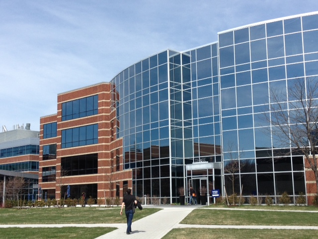
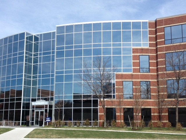
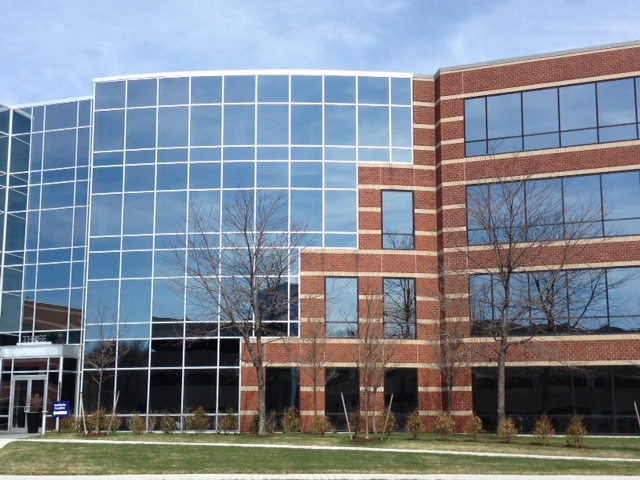
And recreate a big image looking like this:

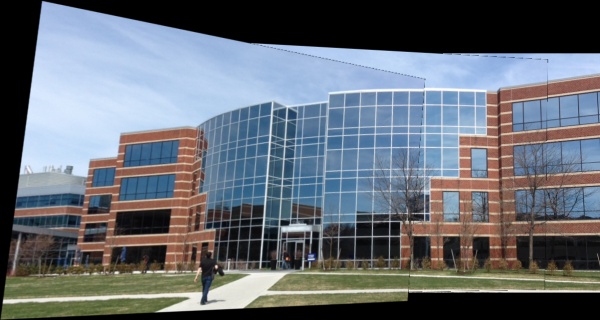
To do this, we will use OpenCV (imported as cv2), which is one of the most popular and powerful computer vision libraries in the world. While you will need to learn how to install OpenCV on your own personal computer, you do not need to worry about that right now. In the CodeSignal environment, OpenCV and all other necessary tools come pre-installed and ready to use!

Also, you will have a small Image Gallery to help you debug your work along the exercises!

Before we dive deeper into the code, it is important to understand what a digital image actually is. To our eyes, it’s a photograph, but to a computer, it is a three-dimensional grid of numbers, also known as a multidimensional array.

• Pixels: The grid is made up of individual dots called pixels. Every pixel in the image contains numerical data that tells the computer what color to display.
• Spatial Dimensions: The first two dimensions of this grid represent the height and width of the image (the number of pixels stacked vertically and horizontally).
• Channels: The third dimension represents color channels.

In digital imaging, colors are created by mixing primary colors of light. Most images use the RGB color model, which consists of three channels: Red, Green, and Blue.

Think of these channels as three separate grayscale layers. When you stack them on top of each other, they blend to create a full-color image. Each pixel in a standard 8-bit image has a value for each channel ranging from 0 (no intensity) to 255 (full intensity). For example:

• A pixel with values (255, 0, 0) in RGB is pure Red.
• A pixel with (0, 0, 0) is Black (all lights off).
• A pixel with (255, 255, 255) is White (all colors at maximum intensity).

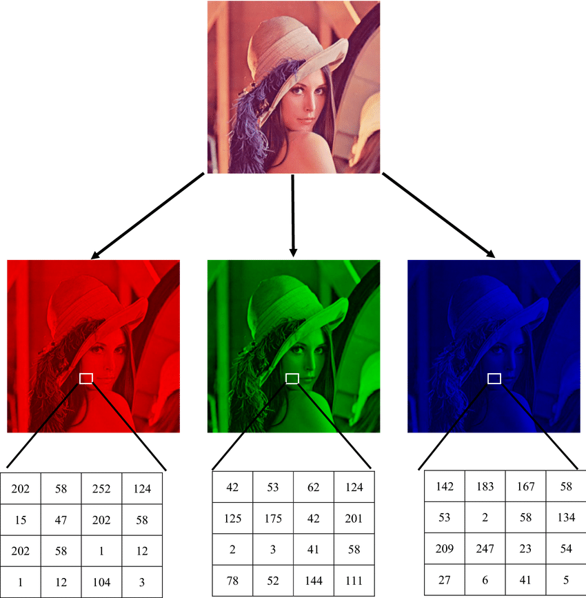
The OpenCV Difference: While the world usually uses RGB, OpenCV reads images in BGR (Blue-Green-Red) order. This means the first layer of data is Blue, the second is Green, and the third is Red. We must keep this in mind whenever we manipulate individual color values!

Let's start by setting up a way to tell our Python script which image we want to load. We can use Python's built-in argparse library to read command-line arguments. This allows us to pass a file path and other options directly into our program.

import argparse
import cv2

def main():
    parser = argparse.ArgumentParser()
    parser.add_argument("path")
    parser.add_argument("--out", default="")
    parser.add_argument("--preview-size", type=int, default=900)
    args = parser.parse_args()

In this code, we expect the user to provide a path to the image. We also set up optional arguments for saving an output file (--out) and setting a maximum window size for our screen (--preview-size).

Next, we need to load the image into our program. We do this using cv2.imread().

    image = cv2.imread(args.path)
    
    if image is None:
        raise SystemExit(f"Could not read image: {args.path}")

Here, cv2.imread() attempts to read the file. If the file path is incorrect or the file is corrupted, OpenCV will not crash immediately; instead, it simply returns None. Therefore, it is very important to include a safety check. If the image is None, we stop the program and print a helpful error message so that we know exactly what went wrong.

To a computer, an image is not a picture; it is simply a massive grid of numbers known as an array. Let's add some code to inspect the mathematical properties of our newly loaded image.

    print("shape:", image.shape)
    print("dtype:", image.dtype)
    print("min/max:", image.min(), image.max())
    print("note: OpenCV loads color images as BGR, not RGB")

Let's break down what these properties tell us:

• shape: This tells us the dimensions of the image. For a color image, it returns three numbers: height, width, and color channels.
• dtype: This is the data type. Typically, it is uint8, which stands for an 8-bit unsigned integer.
• min and max: These are the lowest and highest pixel values in the image grid. Because we are using 8-bit integers, the lowest possible value is 0 (pure black) and the highest is 255 (pure white or full color).

If you were to run this code on a standard photo, you would see output that looks something like this:

shape: (4000, 6000, 3)
dtype: uint8
min/max: 0 255
note: OpenCV loads color images as BGR, not RGB

Note the warning we printed at the end! By default, almost all computer graphics use Red-Green-Blue (RGB) order for colors. However, OpenCV has a famous quirk: it loads colors in Blue-Green-Red (BGR) order. It is very helpful to print this reminder so that we do not forget it later.

If you look at the sample output above, the image has a height of 4000 pixels and a width of 6000 pixels. Modern photos are huge! If we try to show this image on a standard computer monitor pixel-for-pixel, it will be much larger than the screen.

To fix this, we will write a custom helper function to shrink the image specifically for our preview window.

def resize_long_edge(image, max_size=900):
    height, width = image.shape[:2]
    scale = min(1.0, max_size / max(height, width))
    
    if scale == 1.0:
        return image.copy()
        
    return cv2.resize(image, (int(width * scale), int(height * scale)))

Let's explain the math behind this step by step:

1. First, we examine the image shape to get the height and width.
2. Next, we determine which side is the longest using max(height, width).
3. We divide our target max_size (which defaults to 900 pixels) by that longest edge to find our scale percentage. For example, if the image is 1800 pixels wide, 900 / 1800 gives us a scale of 0.5 (or 50%).
4. We use min(1.0, ...) to ensure that if the image is already smaller than 900 pixels, our scale remains at 1.0. We do not want to stretch small images.
5. Finally, we use cv2.resize() to shrink the image to its new dimensions.

It is crucial to note that this resizing is strictly for our display screen. We want to keep the original, high-quality image array untouched for our actual stitching work later.

Now that we have our original image loaded and a handy resize_long_edge function ready, let's complete our main() function by displaying the image to the user.

    if args.out:
        cv2.imwrite(args.out, image)

    cv2.imshow("preview", resize_long_edge(image, max_size=args.preview_size))
    cv2.waitKey(0)
    cv2.destroyAllWindows()

if __name__ == "__main__":
    main()

Here is what these final few lines do:

• First, we check if the user provided an --out argument. If they did, we use cv2.imwrite() to save a copy of the full-resolution image to their computer.
• Next, we use cv2.imshow(). This command usually creates a pop-up window named "preview" and displays the result of our resize_long_edge function, but in the CodeSignal environment it will be displayed on the Image Gallery.
• Crucial Step: We must call cv2.waitKey(0). This tells Python to pause the program indefinitely (where 0 signifies forever) until the user presses a key on their keyboard. In our case, a button will appear on the Image Gallery to let the program continue. If we forget this line, the window will appear and disappear in a fraction of a second before we can even see it!
• Finally, once the user presses a key, cv2.destroyAllWindows() safely closes the preview window and cleans up the program. In our CodeSignal IDE this will destroy all images inside the Image Gallery.

Excellent work! We have successfully built the foundation for our workbench. We learned how to use command-line arguments to pass in a file path, and we used cv2.imread() to read the image into our program. We explored how to inspect the mathematical properties of the image array, such as its shape and data type. Finally, we created a custom mathematical helper function to resize the image, and we used cv2.imshow() and cv2.waitKey(0) to safely display it on our screen.

You are now ready to put these concepts to work. In the upcoming interactive exercises, you will practice writing these loading, inspecting, and display functions yourself. Becoming comfortable with these basic OpenCV tools now will make it much easier when we move on to the complex math and stitching algorithms in the next lessons!