Welcome back! In our previous units, we built our workbench tools. We learned how to read color images using our read_color function and how to inspect them side-by-side using make_panel. Now, we are entering Unit 3, where we need to prepare our images so that the computer can find matching points between them.

When we stitch images together to make a panorama, our program needs to find common points — called "features" — in both images. Feature detectors look for distinct shapes, corners, and edges. They do not care about colors, and they struggle if an image is too dark, washed out, or grainy.

In this lesson, we will build a preprocess_for_features function. Our goal is to convert images to grayscale, boost their contrast, and smooth out any distracting noise. By the way, we will be using the OpenCV (cv2) library for this. In the CodeSignal environment, this library comes pre-installed, so you do not need to worry about setting it up right now.

Feature detectors process images using complex math. Full-color images have three channels (Blue, Green, and Red), which means three times the amount of data to process. To simplify the math and speed up our program, our first step is always to drop the colors.

Let's start building our preprocessing function by converting the input image to grayscale using OpenCV's cv2.cvtColor function.

import cv2

def preprocess_for_features(image):
    # Convert the BGR color image to a single-channel grayscale image
    gray = cv2.cvtColor(image, cv2.COLOR_BGR2GRAY)
    
    return gray

If you were to check the shape of your image matrix before and after this step, a color image might look like (900, 1200, 3), while the output gray image would be just (900, 1200). This simpler format is exactly what our feature detectors expect.

Sometimes images are flat or have low contrast, making it difficult to find distinct corners. To fix this, we can boost the contrast.

Instead of boosting the contrast across the whole image (which might wash out bright areas and darken shadows), we use a tool called CLAHE (Contrast Limited Adaptive Histogram Equalization).

To understand CLAHE, we first need to understand two basic concepts:

1. Histogram: Imagine a bar chart that counts how many pixels of each brightness level exist in an image—from pure black on the left to pure white on the right. This is a histogram. If a photo is "flat" or low-contrast, all the bars will be bunched up in the middle.
2. Histogram Equalization: This is a technique that takes those bunched-up bars and "stretches" them out across the entire range. This makes the darks darker and the lights lighter, forcing details to become more visible.

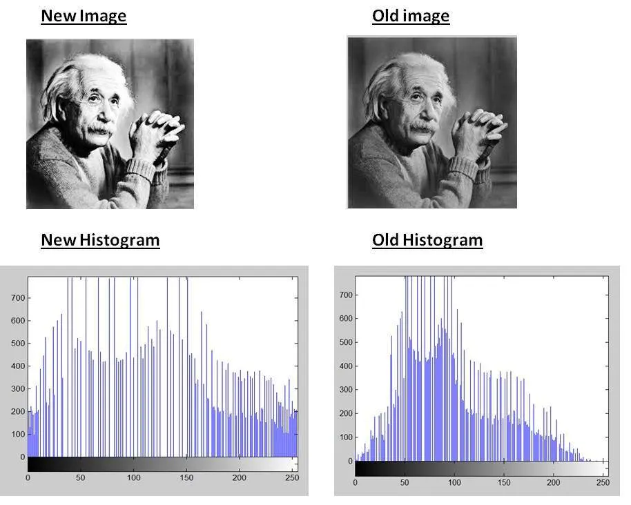
CLAHE improves on this with two main principles:

• Adaptive (Local): Instead of looking at the histogram of the entire image (which might over-brighten a sky just to see a dark building), CLAHE divides the image into small tiles (like an 8x8 grid). It calculates and stretches the contrast for each tile individually.
• Contrast Limited: In areas with no detail (like a clear sky), standard equalization can accidentally amplify tiny bits of digital sensor noise until they look like ugly grain. The "clip limit" caps the boost, ensuring we only enhance real features and keep the background clean.

Let's update our function to include optional CLAHE processing. We will use a clipLimit of 3.0 to boost contrast and a tileGridSize of 8 to divide the image into an 8x8 grid.

import cv2

def preprocess_for_features(
    image,
    use_clahe=True,
    clahe_clip_limit=3.0,
    clahe_tile_grid_size=8,
):
    gray = cv2.cvtColor(image, cv2.COLOR_BGR2GRAY)

    if use_clahe:
        # Ensure our grid size is at least 1
        tile_size = max(1, int(clahe_tile_grid_size))
        
        # Create the CLAHE tool with our specific settings
        clahe = cv2.createCLAHE(
            clipLimit=clahe_clip_limit,
            tileGridSize=(tile_size, tile_size),
        )
        
        # Apply the contrast boost to our grayscale image
        gray = clahe.apply(gray)

    return gray

Cameras sometimes produce grainy images, especially in low light. A feature detector might get confused and think a random speck of digital noise is a valuable corner or edge. To prevent this, we can apply a slight blur to smooth out the image.

Gaussian Blur is a technique used to reduce image noise and detail. Unlike a simple blur that averages all pixels in a neighborhood equally, a Gaussian blur uses a "weighted average." It follows a Gaussian distribution (a bell-shaped curve), where the pixel at the center has the highest weight, and pixels further away have less influence. This results in a "softer" image that removes high-frequency noise while preserving the overall structure.

To apply this blur, OpenCV uses something called a kernel. Think of a kernel as a small square window (a matrix) that slides over every pixel in your image.

1. The kernel centers itself over a pixel.
2. It looks at the neighboring pixels within the window.
3. It performs a mathematical calculation (the weighted average) to determine the new value for that center pixel.
4. It moves to the next pixel and repeats the process.

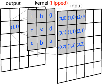
For this math to work correctly, the kernel needs a single, clear center pixel. This is why OpenCV has a strict rule: the blur_size (the width and height of the kernel) must be an odd number, like 3x3, 5x5, or 7x7. If we pass an even number, OpenCV cannot find a perfect center, and the program will crash. We will add a simple check to automatically add 1 to any even number to keep things safe.

For pixels on the edges, the kernel window would hang off the image. OpenCV handles this by using border padding—it essentially creates "virtual" pixels outside the boundary (often by reflecting the inner pixels) so the math can still work.

Let's add the blurring logic to our function.

import cv2

def preprocess_for_features(
    image,
    use_clahe=True,
    blur_size=0,
    clahe_clip_limit=3.0,
    clahe_tile_grid_size=8,
):
    gray = cv2.cvtColor(image, cv2.COLOR_BGR2GRAY)

    if use_clahe:
        tile_size = max(1, int(clahe_tile_grid_size))
        clahe = cv2.createCLAHE(
            clipLimit=clahe_clip_limit,
            tileGridSize=(tile_size, tile_size),
        )
        gray = clahe.apply(gray)

    # Only apply blur if a size greater than 0 is requested
    if blur_size > 0:
        # OpenCV requires odd kernel sizes to have a center pixel. 
        # If even, make it odd.
        if blur_size % 2 == 0:
            blur_size += 1
            
        # Apply the Gaussian blur with the specified kernel size
        # (blur_size, blur_size) defines the width and height of the kernel
        gray = cv2.GaussianBlur(gray, (blur_size, blur_size), 0)

    return gray

We now have a complete, robust preprocess_for_features function! It takes an image, strips away the distracting colors, boosts the hidden details, and smooths out the noisy grain.

To see how this fits into the bigger picture, here is a quick look at how you might use this new function alongside the tools we built in previous units. We load the image, preprocess it, and display the original next to the prepared version using our make_panel tool.

# Assuming read_color and make_panel are imported from our toolkit
image = read_color("photo.jpg")

# Prepare the image using our new function
prepared = preprocess_for_features(
    image,
    use_clahe=True,
    blur_size=3
)

# Display the original color image and the prepared grayscale image side-by-side
panel = make_panel(
    [
        ("original", image),
        ("feature input", prepared),
    ],
    max_size=900,
)

cv2.imshow("preprocessing", panel)
cv2.waitKey(0)
cv2.destroyAllWindows()

When you run code like this, a window will pop up showing your original color image on the left and a crisp, high-contrast grayscale version on the right — ready for feature detection!

Now, it is your turn. In the upcoming practice exercises, you will write this preprocessing logic yourself and integrate it into our growing stitching workbench. Let's jump into the code!